This post provides an analysis demo using flights data in R. The source data includes information on over 7.2 million scheduled non-stop U.S. domestic flights during 2018. Given the data’s large size, the DBI package will be used to access a SQLite database where the data is stored. That way, database queries can be generated outside of R without having to bring in the entire dataset as an object.
To make it even more manageable, the focus will be on my hometown airport: McCarran International Airport (LAS), the main airport servicing the Las Vegas metro area. The queries will summarize flight activity and key on-time performance measures: cancellations and flight delays. Findings will be displayed via tables and charts.
For convenience, R codes are available throughout and are also available in its entirety (including code for generating further data manipulation, chart, and table tasks) on my GitHub.
=======
R provides various ways to access Comma Separated Values (CSV) files. CSV files are in a plain text format designed to easily exchange data between different applications. An easy way to import the data from a CSV file into R and keep the object in memory is to use the built-in read.csv function.
Alternatively, if the CSV file is already stored as a table in an outside relational database, R can likely access the data since it can connect to almost any database type. A common method to do this is through the use of the DBI (DataBase Interface) package, a database interface definition for communicating between R and a relational database management system (DBMS). Among them is SQLite, a light-weight, open source database engine.
Since I currently store large data sets in my private SQLite DBMS, I opted for the latter option. That way, rather than reading in the entire data set, I can use Structured Query Language (SQL) statements to retrieve smaller chunks of data needed for the specific analysis at hand. This can be useful - necessary even - when handling very large data sets on personal computers with memory limitations.
The subject data for this post is on arrival and departure information for non-stop domestic flights during 2018, by airline carrier and by airport (both origin and destination). Considering that these airlines together make nearly 20,000 flight trips each day throughout nearly 360 airports nationwide, they provide sizable metadata for the data analytics community looking to practice on larger data sets. The data is used widely to test out statistical inference models and predictive machine learning algorithms.
All the data will not be used since the focus will be on answering a series of questions about flight activity and on-time performance for a single airport: McCarran International Airport (LAS), the main airport in the Las Vegas, Nevada metro area. Furthermore, the aim here is not so much about applying advanced analytical techniques. It will be simpler than that: to practice SQL queries to get the data needed to perform basic summaries that generate insight into LAS. Lastly, since exhibits are an effective way to succinctly report findings, the questions will be answered through corresponding charts and tables.
Thus, the learning goals covered here will be to:
- Access a database and run SQL queries in R (using DBI & RSQLite ), and
- Summarize the data and generate exhibits for each query.
1. About the Data
Commercial airline carriers report the flights information to the U.S. Department of Transportation’s Bureau of Transportation Statistics (BTS). The publicly-available source data was abridged and extracted as a set of plain-text CSV files. The data was then loaded into a SQLite database and saved as “flights2018.db”.
The “flights2018.db” database schema consists of four tables:
- flights (month, dayofwk, carrier, origin, dest, num_flights, cancelled, dep_del, dep_del15, arr_del, arr_del15, distance, ad_carrier, ad_weather, ad_nas, ad_security, ad_lateaircraft)
- airports (code, city_name, airport_name)
- carriers (code, carrier_name)
- days (code, day)
The main table is flights, and we’ll go over the details for all the columns in a bit. For now, note that the names of the airport (“origin” and “dest”), airline carrier (“carrier”), and day (“dayofwk”) for a scheduled flight are not explicitly given. Instead, they contain a code that will be used to join the related tables that provide the names as follows:
- both
flights.originandflights.destreferenceairports.code flights.carrierreferencescarrier.codeflights.dayofwkreferencesdays.code
2. Connecting to SQLite
In order to interact with SQLite, we need to bring in RSQLite, the package that embeds SQLite in R. It will serve as a backend extension to DBI. (In addition to SQLite, other DBI-compliant DBMS types include MonetDB, MySQL, PostgreSQL.) Common DBI functions will be used to connect to SQLite, execute statements from there, and retrieve results from the statements into R.
DBI is installed with RSQLite so there is no need to install it separately.
install.packages("RSQLite")
After installation, the packages’ libraries will be loaded into the R environment. DBI will be loaded first, not RSQLite, since the functions to be used will primarily come from DBI.
library(DBI)
library(RSQLite)
Connection to the database is made through the function call dbConnect().
# Connect to database
## note: generated on my local computer & connected to my local SQLite)
db <- dbConnect(RSQLite::SQLite(), dbname = "flights2018.db")
The first parameter is the name of the DBMS to connect to: SQLite().
The second is the name of the database file, given as dbname = flights2018.db. R uses the current working directory contained in getwd() to find the database file by default, or will otherwise need a full directory path that leads to it. Lastly, this connection is assigned to a variable name “db”, which will be used in the codes throughout the rest of this post.
Check tables
From here, we can check whether we are accessing the database file correctly with the dblistTable function. We simply pass the database connection name through it.
dbListTables(db)
## [1] "airports" "carriers" "days" "flights"
As expected, all four tables are accessible and available for interaction within the R environment.
Check fields
How about the column (field) names in the flights table? We can use dbListFields() to list them all.
dbListFields(db, "flights")
##  [1] "month"           "dayofwk"         "carrier"
##  [4] "origin"          "dest"            "num_flights"
##  [7] "cancelled"       "dep_del"         "dep_del15"
## [10] "arr_del"         "arr_del15"       "distance"
## [13] "ad_carrier"      "ad_weather"      "ad_nas"
## [16] "ad_security"     "ad_lateaircraft"
Definitions
These 17 fields contain the following information:
- month and dayofwk: dates of a scheduled flight, beginning with 1 for January (months) and 1 for Monday (day of week).
- carrier: code assigned by IATA to identify an airline carrier.
- origin and dest: code assigned by U.S. DOT to identify a flight’s origin and destination airports, respectively.
- num_flights: equal to 1 since each entry corresponds to a single flight.
- cancelled: indicator for whether a scheduled flight was cancelled (1 = cancelled).
- dep_del and arr_del: minutes delayed at departure and at arrival, respectively, measured as the difference between scheduled and actual times (negative values = early).
- dep_del15 and arr_del15: indicator for whether the departure and arrival was delayed by 15 minutes or more (1 = delayed).
- distance: distance in air miles between a flight’s origin and destination airports.
- ad_carrier, ad_weather, ad_nas, ad_security, and ad_lateaircraft: minutes contributed to arrival delay(s), reason(s) due to a carrier, weather, National Aviation System, airport security, and late-arriving aircraft, respectively (0 or more only when arr_del15 = 1, NA otherwise)
3. Research Questions
The data in the flights table provide for the development of a lot of interesting questions. The ones to address here include the following:
- What were the busiest days of the week and months of the year at LAS?
- What were the most popular cities paired with LAS (both directions to and from)?
- How well did LAS perform when it came to on-time measures (cancellations and delays)?
- What were the main reasons for flight delays from LAS?
4. Applying SQL Statements
At this point, we’ve connected to a database, checked all the tables are in, defined the contents in the flights table, and come up with some general questions to explore. In this section, we move on to how SQL statements can be used in R through written queries. Most will be simple, with a few complex nested ones, in order to arrange the data (e.g., filter, group, summarize, sort, etc.). We won’t go over all the different types of SQL statements, but suffice to say we will use SELECT, ALTER, and UPDATE to query the database.
dbGetQuery
As a starter, let’s write a query to get a count of the rows in the flights table. Passing a SELECT statement through the dbGetQuery function from DBI will interact with the database to both execute the query and retrieve the set of data.
dbGetQuery(db, "SELECT COUNT(*) FROM flights")
##   COUNT(*)
## 1  7213446
This returned a result of 7.2 million rows. We can get just the first 10 rows of the table and assign it to a variable called “getPreview”. Note that this will return a data frame object with as many rows fetched (10 records) and as many columns in the result set (17 fields).
getPreview <- dbGetQuery(db, "SELECT *
                         FROM flights
                         LIMIT 10;")

getPreview
##    month dayofwk carrier origin dest num_flights cancelled dep_del
## 1      1       6      UA    FLL  IAH           1         0     -13
## 2      1       6      UA    SEA  SFO           1         0      -4
## 3      1       6      UA    DCA  IAH           1         0      -2
## 4      1       6      UA    LAX  ORD           1         0      -9
## 5      1       6      UA    JAX  EWR           1         0     -14
## 6      1       6      UA    IAH  PHX           1         0      -7
## 7      1       6      UA    EWR  HNL           1         0      27
## 8      1       6      UA    HNL  EWR           1         0       8
## 9      1       6      UA    LAS  SFO           1         0      -5
## 10     1       6      UA    IAD  TPA           1         0      -7
##    dep_del15 arr_del arr_del15 distance ad_carrier ad_weather ad_nas
## 1          0     -12         0      966         NA         NA     NA
## 2          0     -18         0      679         NA         NA     NA
## 3          0       1         0     1208         NA         NA     NA
## 4          0      -8         0     1744         NA         NA     NA
## 5          0     -24         0      820         NA         NA     NA
## 6          0     -19         0     1009         NA         NA     NA
## 7          1      19         1     4962          0          0      0
## 8          0     -23         0     4962         NA         NA     NA
## 9          0     -22         0      414         NA         NA     NA
## 10         0     -18         0      811         NA         NA     NA
##    ad_security ad_lateaircraft
## 1           NA              NA
## 2           NA              NA
## 3           NA              NA
## 4           NA              NA
## 5           NA              NA
## 6           NA              NA
## 7            0              19
## 8           NA              NA
## 9           NA              NA
## 10          NA              NA
We can also clarify the type of data we’re looking at for each field (e.g., stored as character, integer, date, or Boolean values) and document it by assigning it as “getDatatype”.
getDatatype <- dbGetQuery(db, "SELECT cid,
       name AS field_name,
       type AS data_type
  FROM PRAGMA_table_info('flights');")

getDatatype
##    cid      field_name data_type
## 1    0           month      DATE
## 2    1         dayofwk      DATE
## 3    2         carrier   VARCHAR
## 4    3          origin   VARCHAR
## 5    4            dest   VARCHAR
## 6    5     num_flights   INTEGER
## 7    6       cancelled   BOOLEAN
## 8    7         dep_del   INTEGER
## 9    8       dep_del15   BOOLEAN
## 10   9         arr_del   INTEGER
## 11  10       arr_del15   BOOLEAN
## 12  11        distance   INTEGER
## 13  12      ad_carrier   INTEGER
## 14  13      ad_weather   INTEGER
## 15  14          ad_nas   INTEGER
## 16  15     ad_security   INTEGER
## 17  16 ad_lateaircraft   INTEGER
dbExecute
So far, we’ve applied SELECT statements, which is the only type dbGetQuery() takes. In instances when there is no need to retrieve a result set after executing a query, the dbExecute function will be used. This is for data modification statements such as ALTER (to modify the structure of a table) or UPDATE (to modify the data stored in a table). It will be needed later for data definition and data manipulation purposes.
These two DBI functions are enough for our purposes, but there’s more documented in the vignette available here should you want to explore them.
5. Exploring Flights Data for LAS
In this section, we intend to answer our research questions related to LAS by extracting the necessary chunks of data using queries and transforming them into exhibits.
The research questions have been developed into 10 specific ones, half concerning flight activity at LAS (Part A) and the other half concerning on-time performance to the top 10 destinations from LAS (Part B).
Part A: Flight Activity at LAS
Q1. Which airports were the busiest, and where did LAS rank?
# QUERY
q1_fltAirp <- dbGetQuery(db, "SELECT s1.Airport AS AirportCode,
       s1.FlightsAsOrigin,
       final.FlightsAsDest,
       s1.FlightsAsOrigin + final.FlightsAsDest AS TotalFlights
  FROM (
           SELECT airports.code AS Airport,
                  origin,
                  SUM(num_flights) AS FlightsAsOrigin
             FROM flights
                  INNER JOIN
                  airports ON origin = code
            GROUP BY origin
       )
       AS s1
       LEFT JOIN
       (
           SELECT *
             FROM (
                      SELECT dest,
                             SUM(num_flights) AS FlightsAsDest
                        FROM flights
                             INNER JOIN
                             airports ON dest = code
                       GROUP BY dest
                  )
                  AS s2
       )
       AS final ON s1.origin = final.dest
 ORDER BY TotalFlights DESC
 LIMIT 20;")
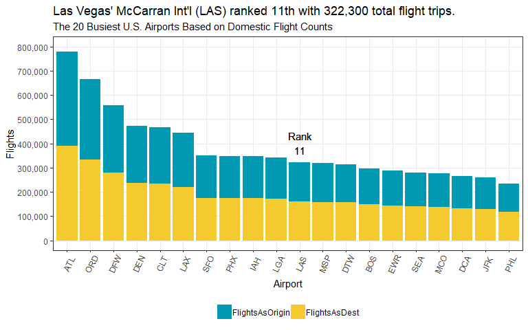
The chart below shows the top 20 busiest U.S. airports, based on the number of scheduled flights serviced (in both directions, as the origin and destination) on an annual basis. Without information on passenger count and seat capacity, we miss a complete picture of how busy an airport really is. Regardless of how it could be measured, ATL (Hartsfield-Jackson Atlanta) takes the top spot by far. No surprise here; ATL has held this rank for over the past decade. ORD (Chicago O’Hare) trails second, followed by DFW (Dallas/Fort Worth).
Where does LAS come in? In 11th place, handling over 322,000 flights. The Las Vegas metro area is home to only ~2.2 million residents, the smallest population amongst all the metro areas serviced by these top airports, so LAS’ rank is heavily driven by the region’s tourism-based economy.
Q2. When were the busiest months for travel at LAS?
# QUERY
q2_fltMonth <- dbGetQuery(db, "SELECT month,
       SUM(num_flights) AS num_flights
  FROM flights
 WHERE dest = 'LAS' OR
       origin = 'LAS'
 GROUP BY month
 ORDER BY num_flights;")
Tourism levels can vary significantly depending on the type of vacation and business destination a region is considered to be. For Las Vegas, the city attracts visitors year round, so it does not have well-defined high and low tourism seasons.
This is reflected in the chart below, where the number of scheduled flights were fairly consistent from month to month. An exception was February, when there was a noticeable drop in flight activity. However, this is generally true for airports throughout the U.S. in general. Also, October saw an uptick from the previous month, but it should be compared to other years to determine if it was an aberration.

Q3. What were the busiest days of the week at LAS?
# QUERY
q3_fltDay <- dbGetQuery(db, "SELECT dayofwk,
       days.day AS day,
       SUM(num_flights) AS num_flights
  FROM flights
       LEFT JOIN
       days ON flights.dayofwk = days.code
 WHERE origin = 'LAS' OR
       dest = 'LAS'
 GROUP BY dayofwk;")
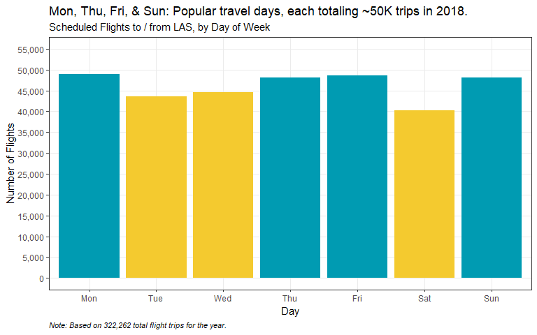
Mondays, Thursdays, Fridays, and Sundays were likewise the busiest days in terms of scheduled flights to and from LAS.
Saturday was the least busy. Since it’s in the middle of the “weekend” (when defined as Friday to Sunday), it makes sense that Saturday would not be the ideal day to leave for or return from a Las Vegas trip. Similarly, the middle of the “weekday” (Tuesdays and Wednesdays) were relatively slower.
Overall, the pattern is consistent with the reported average length of stay of visitors during 2018, which was 3.4 nights and 4.4 days according to the LVCVA.
Q4. Which airline carriers serviced the most flights at LAS?
There were 12 airline carriers operating out of LAS during 2018. This is now down to 11 carriers since the Virgin America merger with Alaska Airlines. Virgin reported independently for the first three months of last year until April, when it began reporting jointly as Alaska Airlines.
An UPDATE query modifies the data stored in a table. An asterisk (“*”) is added to denote this merger in the chart below.
# QUERY
dbExecute(db, "UPDATE carriers
   SET carrier_name = '*Virgin America'
 WHERE code = 'VX';") #--Add * for footnote on VX merger
# QUERY
q4_fltCarr <- dbGetQuery(db, "SELECT carriers.carrier_name,
       SUM(num_flights) AS num_flights
  FROM flights
       LEFT JOIN
       carriers ON carrier = code
 WHERE origin = 'LAS' OR
       dest = 'LAS'
 GROUP BY carrier
 ORDER BY num_flights DESC;")
Of the 12 carriers, Southwest Airlines operated the most flights to and from LAS, making it the largest carrier there by a long stretch (46% share). The latest statistics provided by Southwest at the time of this writing reports LAS as the carrier’s third busiest airport in terms of daily departures, serviced across 54 U.S. destinations.

Q5. Most frequent cities paired with LAS flight trips?
Planning a flight trip involves looking up the origin airport and destination airport. The cities where both airports are located is what we mean by “city pairs”.
The ALTER and UPDATE statements will modify the structure and data in the flights table by adding a new column for the city pairs.
# QUERIES
## add empty city pairs field
dbExecute(db, "ALTER TABLE flights ADD city_pairs VARCHAR;")

## fill field with concatenated cities
dbExecute(db, "UPDATE flights
   SET city_pairs = origin || ' , ' || dest;")
# QUERY
q5_fltCityPairs <- dbGetQuery(db, "SELECT *
  FROM (
           SELECT city_pairs AS CityPairs,
                  CASE WHEN origin = 'LAS' THEN 'LAS as Origin' END AS Direction,
                  airports.city_name AS CityName,
                  COUNT(city_pairs) * -1 AS Flights
             FROM flights
                  INNER JOIN
                  airports ON dest = airports.code
            WHERE origin = 'LAS'
            GROUP BY CityPairs
            ORDER BY Flights
            LIMIT 10
       )
UNION ALL
SELECT *
  FROM (
           SELECT city_pairs AS CityPairs,
                  CASE WHEN dest = 'LAS' THEN 'LAS as Destination' END AS Direction,
                  airports.city_name AS CityName,
                  COUNT(city_pairs) AS Flights
             FROM flights
                  INNER JOIN
                  airports ON origin = airports.code
            WHERE dest = 'LAS'
            GROUP BY CityPairs
            ORDER BY Flights DESC
            LIMIT 10
       )
 ORDER BY Flights;")
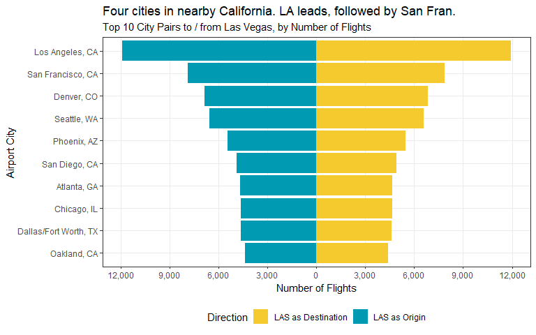
In the chart below, city pairs are shown separately by direction where Las Vegas is either the destination or origin:
- Yellow bars: Frequency of flights where Las Vegas was the destination for each airport city; represented inbound flights into LAS.
- Blue bars: Showed the alternative, where Las Vegas was the origin; represented outbound flights out of LAS. Thus, these can be rephrased as being the “top 10 destinations” (which will be the focus in Part B).
A few comments on the chart above. First, when looking at the degree of outbound flights from Las Vegas (blue) and inbound flights to Las Vegas (yellow), they are practically in-line with each other. A quick check, calculated as: outbound from origin / inbound to destination, shows this to be the case when values are equal to 1.
# PRINT QUERY
dbGetQuery(db, "SELECT s1.CityName, s1.Outbound, final.Inbound,
s1.Outbound * 1.0 / final.Inbound AS Degree

FROM (
  SELECT city_pairs AS 'CityPairsO',
       CASE WHEN origin = 'LAS' THEN COUNT(city_pairs) END AS 'Outbound',
                 airports.city_name AS 'CityName'
                 FROM flights
                 INNER JOIN
                 airports ON dest = airports.code
                 WHERE origin = 'LAS'
                 GROUP BY CityPairsO
                 ORDER BY Outbound DESC
                 LIMIT 10)
AS s1

LEFT JOIN

(SELECT * FROM

(SELECT city_pairs AS 'CityPairsD',
       CASE WHEN dest = 'LAS' THEN COUNT(city_pairs) END AS 'Inbound',
       airports.city_name AS 'CityName'
  FROM flights
       INNER JOIN
       airports ON origin = airports.code
 WHERE dest = 'LAS' AND
origin IN ('LAX', 'SFO', 'DEN', 'SEA', 'PHX', 'SAN', 'ATL', 'ORD', 'DFW', 'OAK')
 GROUP BY CityPairsD)

AS s2)

AS final ON s1.CityName = final.CityName;)")
##                 CityName Outbound Inbound    Degree
## 1        Los Angeles, CA    11927   11948 0.9982424
## 2      San Francisco, CA     7883    7880 1.0003807
## 3             Denver, CO     6861    6838 1.0033636
## 4            Seattle, WA     6567    6566 1.0001523
## 5            Phoenix, AZ     5454    5452 1.0003668
## 6          San Diego, CA     4906    4903 1.0006119
## 7            Atlanta, GA     4668    4667 1.0002143
## 8            Chicago, IL     4640    4639 1.0002156
## 9  Dallas/Fort Worth, TX     4623    4624 0.9997837
## 10           Oakland, CA     4382    4391 0.9979504
Second, it’s important to clarify that the top destinations shown here are within the constraints of the information we have to work with. Recall that the data set represents only non-stop flights in the U.S. (i.e., excludes direct flights that stop, connecting flights that change planes, international flights, etc.). Thus, it provides a limited aspect of city relationships within the broader air travel network.
All these considered, we can say that California is a popular destination, having four of the state’s cities ranking in the top ten. Los Angeles (LAX) tops the list with nearly 12,000 flights from Las Vegas.
In the next part, we’ll look at flight delays and cancellation rates - two important on-time performance measures - for the top ten destinations identified above.
Part B: On-Time Performance to the Top 10 Destinations
First, some definitions. A cancelled flight is self-evident, however the BTS considers a flight to be delayed only when an airline takes off and / or lands later than its scheduled time by 15 minutes or more. We’ll focus just on delays at landing (arrival) for the questions in this part.
Q6. What share of flights were on time versus delayed?
# QUERY
q6_ontPerform <- dbGetQuery(db, "SELECT dest,
       CASE WHEN arr_del15 = '0' THEN 1 END AS [On-Time],
       CASE WHEN arr_del >= '90' OR
                 cancelled = '1' THEN 1 END AS SigDelay,
       CASE WHEN arr_del BETWEEN '15' AND '89' THEN 1 ELSE 0 END AS MinDelay
  FROM flights
 WHERE origin = 'LAS' AND
       dest IN ('LAX', 'SFO', 'DEN', 'SEA', 'PHX', 'SAN', 'ATL', 'ORD', 'DFW', 'OAK');")
The table below shows the overall flight status for all the destinations from LAS. We see that a majority of flights from LAS were punctual, where 80 percent of flights arrived on-time from its scheduled landing (early to less than 15 minutes late). In cases when there were delays, a significant delay (say, an hour and a half or more, and even worse - a cancellation) is considered more consequential than a minor one (less than an hour and a half).
| Arrival Status | Total Flights (#) | Total Flights (%) |
|---|---|---|
| On-Time (early or < 15 min) | 49436 | 80 |
| Significant Delay (>= 90 min or cancelled) | 2598 | 4 |
| Minor Delay (15 - 89 min) | 9877 | 16 |
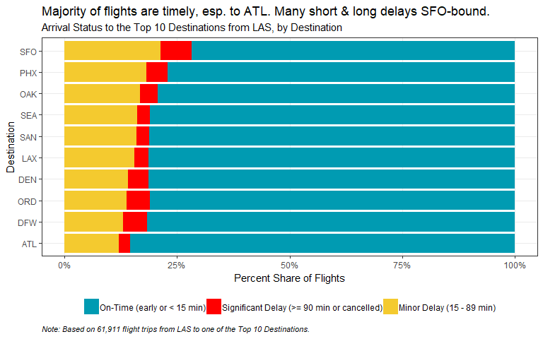
The chart below shows more of the same, except the arrival status is broken down by destination. What’s striking here is that despite being the busiest airport, flights to ATL managed to also be the most timely, having the smallest shares of both delay types. Flights to the two other busiest airports - ORD and DFW - also had a relatively smaller share of its trips delayed, however they were more likely to be significant ones. Meanwhile, on-time performance to SFO (San Francisco International) was the worst, where approximately 30 percent of its flights were delayed to some extent.
Q7. How many minutes can you expect to be delayed?
# QUERY
q7_aDelMin <- dbGetQuery(db, "SELECT dest AS Dest,
       arr_del
  FROM flights
 WHERE arr_del15 = '1' AND
       origin = 'LAS' AND
       dest IN ('LAX', 'SFO', 'DEN', 'SEA', 'PHX', 'SAN', 'ATL', 'ORD', 'DFW', 'OAK')
 ORDER BY dest;")
The previous observations are corroborated with the box plot below. For the delayed flights only, we get a visual of how dispersed the arrival delay minutes were for each destination from LAS.
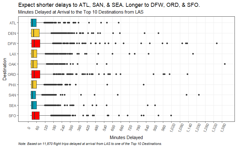
In short, the central rectangle boxes span the interquartile ranges (IQR) from low (Q1) to high (Q3); the vertical line inside marks the median; and the black dots show the outliers (over 1.5 x Q3).
Looking at the hard numbers provided in the corresponding table below, flights to ATL, SAN (San Diego International), and SEA (Seattle-Tacoma International) - when delayed - had the lowest median delay minutes at 32, 31, and 33 minutes, respectively. Taken together with relatively less dispersions from these times, one can conclude that these three airports were the best performers for punctuality.
How about more lackluster performers? This included DFW and ORD, both with a median delay of 44 minutes. These two were very similar in their on-time performance across the board. And, SFO, despite the closer vicinity to LAS, was even worse. You can expect to arrive there 46 minutes late (median). On average, it appeared to do better than DFW and ORD, however this was heavily skewed by the more frequent minor delays.
| Destination | Mean | Minimum | Quartile 1 | Median | Quartile 3 | Maximum |
|---|---|---|---|---|---|---|
| ATL | 53 | 15 | 21 | 32 | 58 | 644 |
| DEN | 65 | 15 | 23 | 39 | 79 | 927 |
| DFW | 82 | 15 | 24 | 44 | 84 | 1343 |
| LAX | 53 | 15 | 22 | 35 | 62 | 1174 |
| OAK | 56 | 15 | 21 | 35 | 64 | 1400 |
| ORD | 78 | 15 | 24 | 44 | 84 | 1133 |
| PHX | 52 | 15 | 23 | 34 | 59 | 821 |
| SAN | 48 | 15 | 21 | 31 | 52 | 1215 |
| SEA | 51 | 15 | 22 | 33 | 60 | 902 |
| SFO | 66 | 15 | 26 | 46 | 80 | 1018 |
Q8. What were the main reasons for the arrival delays?
When a flight is delayed, passengers often look for something to blame. Does one blame extreme weather, security at the airport, or the carrier? All of these are cited as reasons according to the BTS, in addition to two others: air traffic problems (NAS) and late-arriving aircraft. These last two are somewhat ambiguous based on the definitions given directly by the source:
- Air Carrier: The cause of the cancellation or delay was due to circumstances within the airline’s control (e.g. maintenance or crew problems, aircraft cleaning, baggage loading, fueling, etc.).
- Extreme Weather: Significant meteorological conditions (actual or forecasted) that, in the judgment of the carrier, delays or prevents the operation of a flight such as tornado, blizzard or hurricane.
- National Aviation System (NAS): Delays and cancellations attributable to the national aviation system that refer to a broad set of conditions, such as non-extreme weather conditions, airport operations, heavy traffic volume, and air traffic control.
- Security: Delays or cancellations caused by evacuation of a terminal or concourse, re-boarding of aircraft because of security breach, inoperative screening equipment and/or long lines in excess of 29 minutes at screening areas.
- Late-arriving Aircraft: A previous flight with same aircraft arrived late, causing the present flight to depart late.
For instance, within the NAS reason for the delays, there’s a category called “non-extreme weather conditions”. This is reported separately from the Extreme Weather reason, but nonetheless is still related to “blaming the weather”, so to speak.
Also, airline carriers do not report the specific causes for the Late-arriving Aircraft reason. This can mean many things. For example, an aircraft arriving late due to a blizzard can have cascading effects down the air travel network chain, causing the next flight on the same plane to be delayed. Without more information on hand, such as tail numbers for the planes and exact schedule times, we cannot chain together which flights caused the initial late flight delay and why. Thus, when it comes to examining the reasons for arrival delays, it’s within these limitations in mind.
# QUERY
q8_aDelMinReas <- dbGetQuery(db, "SELECT carriers.carrier_name,
       dest,
       ad_carrier AS Carrier,
       ad_weather AS Weather,
       ad_nas AS NAS,
       ad_security AS Security,
       ad_lateaircraft AS [Late-arriving Aircraft]
  FROM flights
       INNER JOIN
       carriers ON flights.carrier = carriers.code
 WHERE arr_del15 = '1' AND
       origin = 'LAS' AND
       dest IN ('LAX', 'SFO', 'DEN', 'SEA', 'PHX', 'SAN', 'ATL', 'ORD', 'DFW', 'OAK');")
Why a flight was delayed could be due to a single reason or a combination of them. The table below provides a breakdown of the contribution each reason made to the total flight delay minutes for the year. Late-arriving Aircraft contributed the most at 42 percent, followed by Carrier and NAS (both at 28 percent). The impact from Weather and Security reasons were negligible.
| Reason | Total Minutes (#) | Total Minutes (%) |
|---|---|---|
| Carrier | 200178 | 28.3 |
| Weather | 8940 | 1.3 |
| NAS | 199050 | 28.1 |
| Security | 577 | 0.1 |
| Late-arriving Aircraft | 299105 | 42.3 |
Perhaps Weather, NAS and Security reasons are harder to control for. The two other reasons - Late-arriving Aircraft and Carrier - may be more variable and in direct control of the airline carrier companies.
We can inquire further which carriers performed better than others depending on the reason(s) why a flight was delayed. It makes sense to also consider the destination airport, since of course not every carrier provided service to all the destinations. Which brings us to our next question.
Q9. What happens when we factor in carriers and airports to the reasons for the delays?
# QUERY
q9_aDelHeat <- dbGetQuery(db, "SELECT carriers.carrier_name,
       dest,
       SUM(ad_carrier) * 1.0 / SUM(arr_del) * 100 AS Carrier,
       SUM(ad_weather) * 1.0 / SUM(arr_del) * 100 AS Weather,
       SUM(ad_nas) * 1.0 / SUM(arr_del) * 100 AS NAS,
       SUM(ad_lateaircraft) * 1.0 / SUM(arr_del) * 100 AS LateAC,
       SUM(ad_security) * 1.0 / SUM(arr_del) * 100 AS Security
  FROM flights
       INNER JOIN
       carriers ON flights.carrier = carriers.code
 WHERE arr_del15 = '1' AND
       origin = 'LAS' AND
       dest IN ('LAX', 'SFO', 'DEN', 'SEA', 'PHX', 'SAN', 'ATL', 'ORD', 'DFW', 'OAK')
 GROUP BY dest,
          carriers.carrier_name
 ORDER BY dest;")
Then we get the chart below. The take-away here? That not all flight delays are equal.
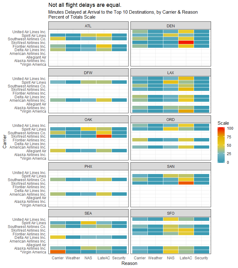
The percent of total minutes that contributed to a flight’s delay for each reason were aggregated and shown on a scale in the range of 0 to 100. A larger value (red) represents a higher percent contributing to a delay, and a smaller one (blue) indicates a lesser percentage. They were broken out by reason and by carrier, for each destination from LAS.
A few observations on the two variable reasons:
Carrier-related
- These were minimal overall across all carriers with routes to SFO and to LAX.
- For the three months Virgin America operated independently, the carrier was severely behind on time when bound for SEA.
- Budget carrier Spirit Air Line’s performance was impressive overall to all of its destinations.
- For the largest carrier - Southwest - performance was relatively worse to its OAK (Oakland International) and ATL bases.
Late Aircraft-related
- There were no significant delay issues attributed to this reason for flights to SEA.
- Conversely, it was the largest driver for delays at LAX, OAK, DEN (Denver International), and SAN (San Diego International).
- SkyWest airlines was especially tardy to these four aforementioned destinations.
- While the biggest culprit of delays to SFO was due to NAS-related problems, late aircraft issues contributed as well.
So far, we’ve focused on arrival delays at landing to the destination, not at departure from the origin. It’s worthwhile to consider the occurrence of departure delays originating from LAS for our last question since the issues described for these two variable reasons happen before takeoff (i.e., due to previous flights, maintenance or crew problems, aircraft cleaning, baggage loading, and fueling).
Q10. How often did delayed flights at departure lead to a subsequent delay at arrival?
A simple way to assess this is to get a count of flights delayed at LAS and from within this set, get a count of flights that were also delayed when arriving to a top destination.
# QUERY
q10_double <- dbGetQuery(db, "SELECT dep_del15,
       arr_del15
  FROM flights
 WHERE dep_del15 = '1' AND
       origin = 'LAS' AND
       dest IN ('LAX', 'SFO', 'DEN', 'SEA', 'PHX', 'SAN', 'ATL', 'ORD', 'DFW', 'OAK');")
Of the ~11,800 delayed flights at departure, 80.4 percent saw a subsequent delay at arrival. The remaining 19.6 percent? They were able to recover. This means that one in five flights were able to make up time in the air and arrive to their destinations on time despite departing late from LAS. Interesting!
## Number of flights:
##  ------------------------------
##  Delayed at departure    11778
##  Delayed at arrival       9468
##      % Delayed at both   80.4%
##  ------------------------------
##  Recovered                2310
##      % Recovered         19.6%
6. Summary
In this post, we demonstrated how to access an outside SQLite database and run queries using the DBI and RSQLite packages. We performed various data manipulation, summarization, and visualization tasks intended to answer a series of questions related to flights activity at LAS and on-time performance to its top destinations.
Of particular interest was our findings that late flights can make up lost time in air. The extent to which this happens is interesting enough that we could come up with a whole other series of questions to explore on this topic alone. In the next post, we’ll do just that and incorporate some statistical regression modeling.
=======
Learning points
-
Although R is extremely fast, the size of the data used with it is limited by RAM available. On my 8 GB 64-bit system, the data slowed down my code runs somewhat. This was resolved through interfacing with a SQLite DBMS (where the data tables were stored) by using DBI and extending it with RSQLite. I was able to generate SQL statements such as SELECT, ALTER, and UPDATE to retrieve the necessary data in chunks. Also, connecting to the database only took a few seconds, a huge improvement over the ~12 minutes required to read in the entire flights data into memory.
-
Aside from covering how to connect to an outside database, our other goal was to answer some questions about flight activity at LAS by getting counts and aggregating. The data showed us that LAS was the 11th busiest airport in the U.S. based on flight counts; travel season was year round; Mondays, Thursdays, Fridays, and Sundays were the busiest days; Southwest Airlines serviced almost half of all flights at LAS; and the top 10 destination airports from LAS included four cities in the neighboring state of California.
-
We then focused on LAS’ on-time performance to its top 10 destinations. Our findings were that a majority of flights arrived on time. At its worst were flights to SFO, where ~30 percent were either cancelled or delayed by at least 15 minutes. When flights did arrive late, the median delay time ranged between 31 minutes minimum (to SAN) and 46 minutes max (to SFO). Late-arriving Aircraft was the biggest determinant of delays, followed by Carrier and NAS-related reasons. However, these reasons should be considered within the context of the different airline carriers and airports. Also, based on the descriptions for the different reasons, it seems that those due to Carrier and Late-arriving Aircraft were largely variable and within the control of the carrier companies to improve efficiencies. The data also revealed an interesting insight: that one in five flights were able to make up time in the air.
-
Lastly, an import aspect of an analyst’s job is to communicate salient findings in a succinct manner. Using data visualization techniques is a powerful way to deliver them. So aside from going through the exercise of generating charts and summary tables for practice, they’re also nice to have.